NYC Taxi Mobility Intelligence

Case study

Many mobility models look accurate because they use information that only becomes available after a trip is complete. I wanted to answer a more realistic question.

I used NYC Taxi & Limousine Commission Yellow Taxi trip records from January through May 2025 and rebuilt the project around this strict prediction-time constraint. Rather than treating it as a retrospective forecasting exercise, the goal was to build a model that could support a user before the trip begins.

Data and validation

To evaluate the model in a realistic future setting, I used a chronological split rather than a random train/test split.

Feature engineering

Information available before departure

The raw NYC TLC dataset contains many highly predictive variables, including actual trip distance, drop-off time, fare components, and payment type. These variables can make a retrospective model look accurate, but they are recorded during or after the trip.

For the production model, I restricted the inputs to information available before departure. From three raw inputs, I engineered a 27-feature pre-trip representation.

Modeling experiments

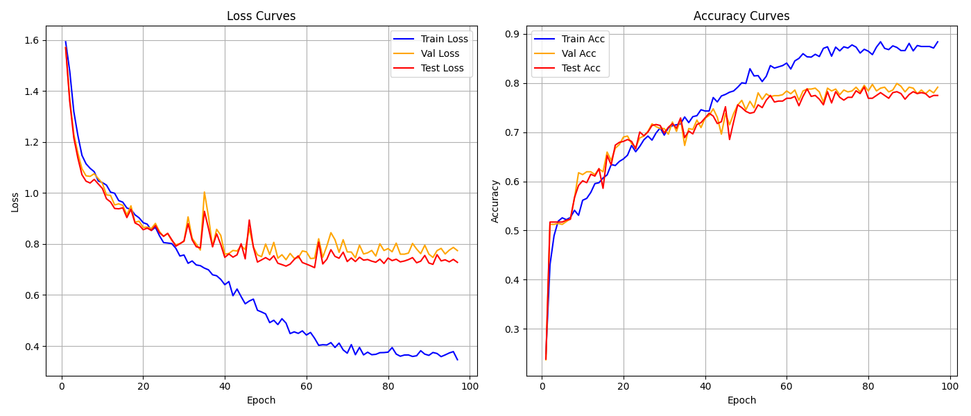
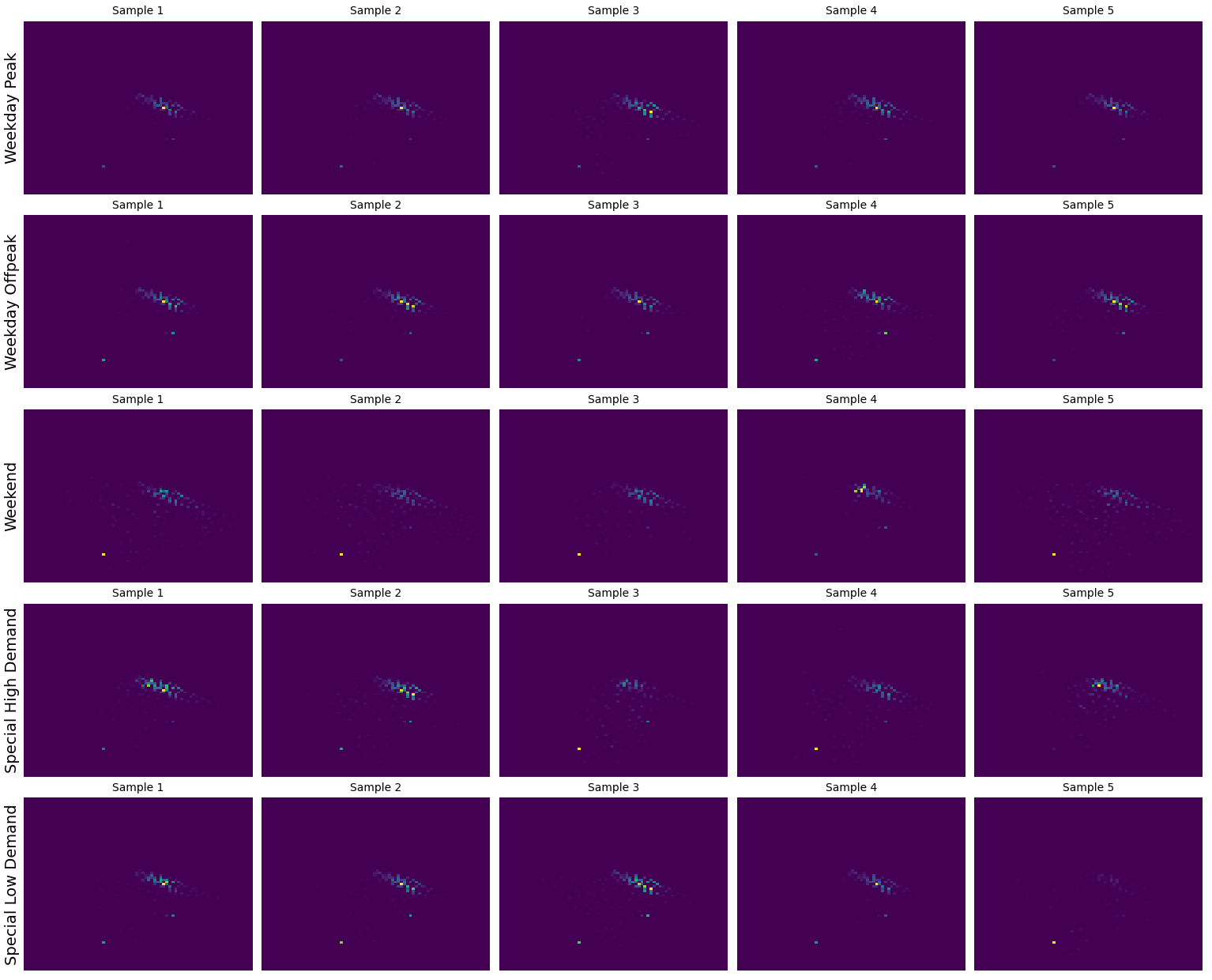
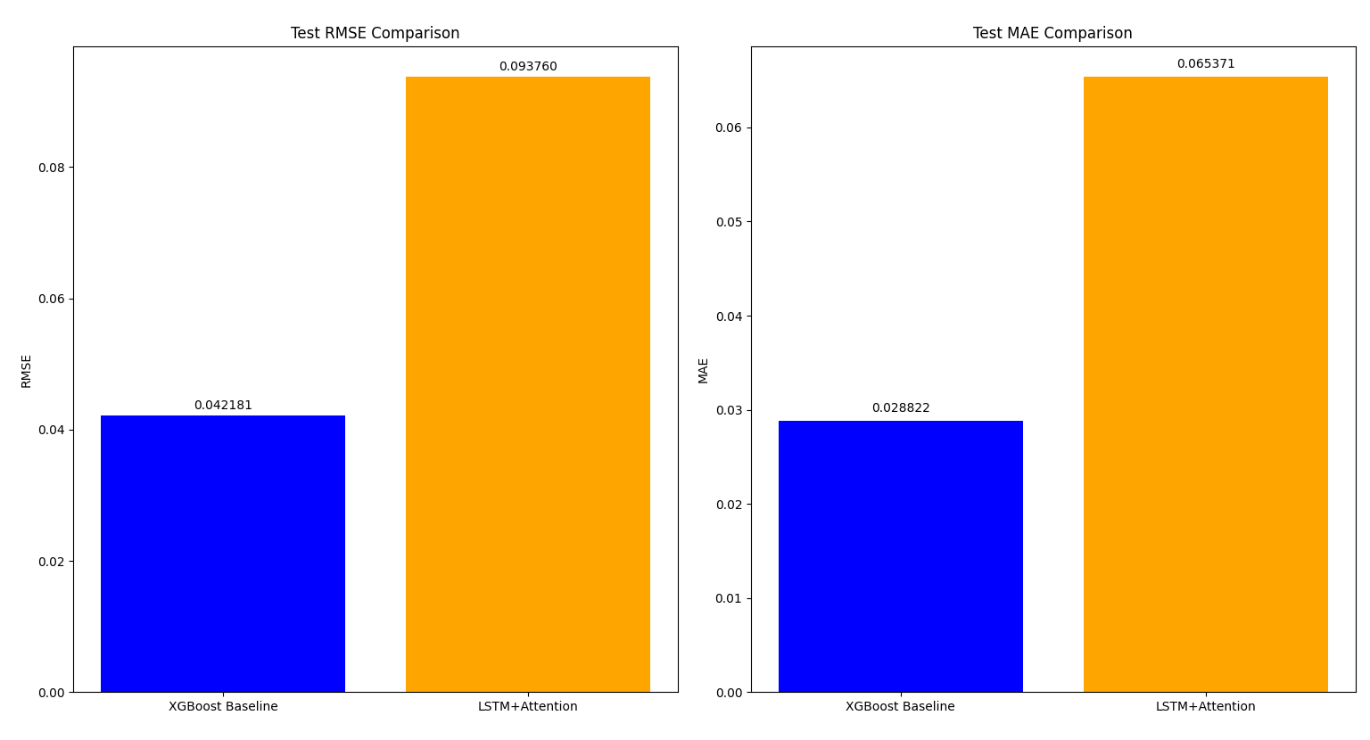
Before deployment, I tried MLP, spatial CNN, Attention-LSTM, and XGBoost models. These experiments explored different representations of taxi behavior, including spatial heatmaps and neural-network architectures.

After auditing the earlier experiments, I found that some results were not directly comparable because they used different feature contracts, random splits, or information that would not exist at prediction time. I therefore rebuilt model selection around the same leakage-safe pre-trip problem.

The lesson was that model selection should follow the structure of the problem rather than the complexity of the architecture.

Model evaluation

I evaluated the models using:

• MAE
• RMSE
• Median absolute error
• P90 absolute error
• P99 absolute error
• Maximum prediction
• Performance on important slices such as airport trips and rare origin–destination pairs

Deployment

I first froze the final XGBoost models and wrapped inference in a FastAPI service. The API converts user-selected locations into coordinates using Google Places, maps those coordinates to canonical TLC Taxi Zones, reconstructs the same 27-feature pre-trip contract used during training, and then runs the frozen models.

I containerized the service with Docker, pushed the image to Google Artifact Registry, and deployed it on Google Cloud Run. Production secrets are stored in Secret Manager, while rate limits, quotas, CORS restrictions, and bounded autoscaling protect the public service.

Google Routes is called separately for route context and is not used as a model input.

Conclusion

The key lesson from this project was that good modeling is not only about accuracy. It is about using the right information, evaluating the model in a realistic future setting, understanding how it fails, and building something that can actually be deployed.